Vacancy Rate and Absorption Rate: A Brief Comparative Review

If you work in real estate research, you most probably understand the significance of vacancy rates and absorption rates when deciding on real estate projects. Albeit, not many real estate investors have a subtle understanding of these two metrics. The purpose of this article is, therefore, to provide a vivid distinction between the use of vacancy rates and absorption rates in real estate. 

Let’s start by simple definitions. Generally speaking, the VACANCY RATE is the percentage of built space in the market currently unoccupied or available for rent. The vacancy rate is determined by considering all the available space for lease and dividing it by the total space in the defined market. to illustrate, let's assume a particular market has 12,500sq. ft. of retail space. Currently, only 625 sq. ft. of retail space available for lease in the market. We divide 625/12,500*100= 5%. We conclude that this market has a 5% vacancy rate for retail units. 

Vacancy Rate= current available space in the market / total number of space in the market *100

Calculating the vacancy rate of a defined market has ample implications. It is often an indicator for developers when to enter or exit the market. If vacancies in the defined market are low, then there is potential demand for new space, which serves as a sign for developers to enter the market and vice versa. Furthermore, lenders also use it for underwriting and feasibility analysts use it to calculate expected returns on a potential project. They take the gross projected revenue and deduct the vacancy rate to determine the effective rental revenues. 

Now, let's focus on the absorption rate. The ABSORPTION RATE is the rate at which homes sell or rent in a given area during a given period of time. In simplistic terms, it is the time (usually defined in months) it would take to sell/rent the currently listed properties in a specific market. Absorption considers both construction of new space and demolition or removal from the market of existing space. It represents the demand over a specified period, contrasted with supply.

We calculate the absorption rate by finding out how many properties are currently available in a specific market. Then, we find out how many property types have been leased or sold (absorbed) within a defined period, we divide the available by the absorbed, and then we have the absorption rate. 

Absorption rate= total number of homes available in the market/ the average number of sales per month

To demonstrate, let’s say there is a total of 120 class-A office spaces in the Downtown Dubai region. After closely observing the market for the last month, we are able to deduct that 40 spaced of class-A office spaces were rented in the area during that period. In accordance with our formula, we divide 12o by 40, which is 3. Therefore, we conclude that there is a three-month supply of class-A office space in the area- A relatively healthy market. 

So what can a real estate developer or investor use this information for? Let’s say you’re a typical investor that wants to lease their Downtown class-A office space 3 months of going into the market. What do you do? If the rent per square foot of class-A office space in the area ranges between $40-$55, you obviously don't list your property at the top end of the range. Rather, you position your space at a discount. In this case, $40 per square foot would guarantee your property will be one of the 40 leased within the next three months. 

Back of the Envelope Analysis: A Pivotal Real Estate Investment Tool

One of the most crucial tools allowing real estate investors to sift through dozens of proposed transactions is the infamous back-of-the-envelope (BOE) analysis. By definition, the BOE is an informal mathematical computation that uses numerical estimations to quickly develop a ‘ballpark figure’. BOE calculations are often used in real estate to determine whether further research and more detailed calculations are warranted.

So, how does the BOE calculation work? Well, it considers the net cash flow of a proposed project and its cap rate. Generally speaking, you will need to make five simple assumptions before commencing the calculation: (i) Purchase price- or initial investment (ii) Rental income- per month or annually (iii) Down payment (iv) Loan amount and term, and (v) Monthly repayment- or amortisation.To illustrate, let’s assume you’re considering investing in a property worth $300,000 and would generate rental income of $595 a week or $2,550 a month. You pay 110,000, borrow $190,000 at 3% a month for 30 years and pay $807 a month.

1) Calculate the annual rent, which is simply the monthly rent multiplied by twelve.

2,550*12= 30,600

2) Calculate cash flow before financing, which is the annual rent (from step 1) multiplied by the operating expenses (let's assume that our operating expenses are 20% here, including property management cost, repair fees, and amenities fees).

30,600*0.80= 24,480

3) Calculate the annual cost of financing, simply the monthly repayment times twelve.

807*12= 9,693

4) Calculate cash flow after financing, which is the cash flow before financing (from step 2) less the annual cost of financing (from step 3).

24,480-9,693= $14,786

after you've completed the above calculations, now you need to compute some key metrics. There are three key metrics that will determine whether a potential investment is worthy: return on asset, cost of financing and return on equity.

Return on asset: Cash flow before financing/price of the property

24,480/300,000= 8%

This is also known as the cap rate. It simply tells you the rate of return the property would produce if you owned it without obtaining a loan/financing.

Cost of financing= annual cost of financing/ loan amount

9,693/190,000= 5%

We usually calculate this figure to compare it to the return on asset figure. If your return on assets is higher than your cost of financing that means you have a positive leverage (which in this case, we do!). In less formal terms, you’re using the bank’s money to generate higher returns than what it cost you to obtain the money.

Return on Equity: cash flow after financing/ equity payment

14,786/ 110,000= 13%

This tells you what your invested equity is earning. When you achieve positive leverage, your return on equity will be higher than your return on assets. Again, in less formal terms, you are earning a higher return by using the bank’s money to finance part of the purchase.

Completing this analysis for the first time might seem time-consuming, but after a couple of tries you get used to it and it becomes a powerful skill to have as a property investor.

After you’ve run the initial analysis (on Excel maybe), you realise how specifically useful this technique is as it allows you to quickly evaluate potential scenarios (think of it as a short-sensitivity analysis). For example, it’ll help you answer questions as ‘what if I borrowed $240,000 for the property instead?’ and ‘how will my returns look if I am able to secure a longer loan period, let’s say 40 years instead’. 

 

                 

In conclusion, the BOE calculation is an approximation method that provides some insight on potential investment projects and NOT a substitute for a fully-fledged analysis. Running the BOE analysis within 5 minutes can give you critical information to decide on which projects are worth looking further into.

Real Estate Financial Modelling: Sensitivity Analysis

A sensitivity analysis, otherwise known as a what-if analysis, constitutes an important tool for decision making in finance. Sensitivity analysis allows financial analysts to foresee what the desired result of a financial model would be under different circumstances.  It is used extensively in real estate to determine how sensitive the outcome is to changes in variable assumptions. 

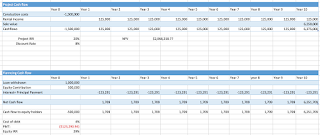
To illustrate, let's refer back to our IRR example from last week. A project that requires an initial investment of $1,500,000 and accumulates an annual rental income of $125,000. After 10 years, the project will be sold for 6,250,000. In this example, $1,000,000 is funded by debt while $500,000 is funded by equity. We find that the project has an IRR of 20% and an equity IRR of 29%. 

                                   
                                    

Here, we are trying to determine how sensitive our IRR analysis is to changes in initial costs or the annual rental revenue (our two main variables). To begin a sensitivity analysis we must first establish a base-case scenario. This is typically the IRR using assumptions we believe to be most accurate. Thereafter, we can change various assumptions we had initially made, based on other potential assumptions. IRR is then recalculated, and the sensitivity of the IRR based on the changes in assumptions is determined. This will be done for both the Project IRR and the Equity IRR.   
                           
To construct the matrix, follow the steps below. 

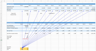
1. Reference your base assumption at 0% sensitivity level. This can be done by simply multiplying all cash flows in your initial IRR analysis by the cells that contain your sensitivity levels. In my preceding example, I added two cells C36 for the base revenue assumption and C37 for the base cost assumption- both at 0%. I then multiplied the initial cash outflow -1,500,00 *(1+C7); likewise, cells D8-M8 have all been multiplied by (1+C36). 

                                   

                                   

                                   

at this step, we are establishing that $1,500,00 is our base cost assumption with a 0% margin of error. Likewise,  $125,000 is our base revenue per year, assuming there is 0% variance in our predictions. 

2. In a cell on the worksheet, reference the formula that refers to the two input cells you want to sensitise. In the example, I referenced my project IRR in cell T66. 

3. Enter one list of input values in the same column, below the formula. In the example, I input a range of development cost possibilities i.e. I expect that the initial cost of construction will vary between -15% (best case) and +15% (worst case).

4. Enter the second list in the same row, to the right of the formula. I have input revenue growth assumptions, which again, I expect to fluctuate between -15% (worst case) and +15% (best case). 

5. Select the range of cells that contains the formula and both the row and column of values. In our example, I have selected T66:AA73.

6.  Click 'What-If analysis' tool under the 'Data Bar'. Select the 'Data table' from the options. Hit Alt-D-T on your keyboard for a shortcut on windows. 

7. In the row input cells box, enter the sensitivity level reference for the row. In my example, the rows represent the revenue income, hence, I selected cell C36 in the row input cell box. 

8. In the column input cells box, enter the sensitivity level reference for the column. In my example, the columns represent the cost of development, hence, I selected cell C37 in the column input cell box. 

9. Press OK! this will give us the different scenarios for the unleveraged IRR!

10. To compute the scenario analysis for leveraged IRR, repeat steps 2-9, just reference the formula for the leveraged IRR as the base cell you want to sensitise. 

                                          

                                           

Spatial Economics: The Rise of Dubai's Commercial Real Estate Market

                          

Before oil was first discovered in Dubai in the late 1960's, the city was a flourishing port for pearl and gold trade, as well as other commercial activities, serving as a major regional hub. After the oil boom of 1973, two years subsequent to the establishment of the United Arab Emirates, the newly-formed federation saw a large inflow of foreign skilled labour, skyrocketing the population of Dubai from 59,000 to 280,000. Expatriates, who comprised 72% of the population at the time, mainly migrated from Europe, North Africa, as well as Southern Asia[1] . 

Soaring oil prices during the early 2000's reinforced momentum to hire large numbers of skilled office workers. From about 61,000 office workers in serviced office buildings in the 1990's, the number of such workers escalated to 123,000 by 2006. The 123,000 workers in 2006 were occupying roughly 15 million square feet (SF) of space in dozens of serviced office towers typically 40 levels high spanning along the world-renowned Shiek Zayed road in the centre of Dubai. The average rent in these buildings was $20/square foot (SF) per year[2].

Figure 1. Office Demand in the Dubai Real Estate Market

The growth in demand is pictured in figure 1. This growth in space demand was caused by the increasing need of work space by office workers. In the early 2000's, the need for space grew drastically due to technological change, such as the increase in popularity of the personal computer and fax machine, resulting in more space necessary per worker [3]. The growth in office demand is represented in Figure 1. by the movement to the right of the demand curve, for example, from a previous time when there were 61,000 workers  (in the 1990s) to the time when there were 123,000 in 2006. To illustrate further, if the need for office workers in downtown Dubai increased further to 180,000 workers, the demand in the market would support an additional 7 million SF of space (a total of 22 million SF would be needed) at the same $20 rent. 

On the other hand, the supply function of real estate is said to be 'kinked'. The supply function is depicted as a vertical line at the current quantity of space supply in the market, which is seen in figure 2. at 10 million SF. This is primarily because the space market is highly inelastic. In other words, if the need for office space falls, the available office space can not be reduced. This can be attributed to the fact that the built space is extremely durable; buildings typically last decades, and refurbishing them is expensive and time-consuming. As a matter of fact, about 98% of supply consists of existing space, while only 2% consists of the flow of new development[4]. The kink in the supply function occurs at the current quantity of built space at a rent level that equates to the long-run marginal cost of supplying additional space to the market. In this case, the marginal cost is simply the cost of developing new buildings, and can be expressed as: 

QS= f(L,N,M,P)

Where the quantity supplied (Qs) is a function of; 
L: the cost of land acquisition
N: the cost of labour employed
M: the cost of building materials
P: a suitable profit margin for developers[5]. 

Hypothetically speaking, for the market to reach equilibrium i.e. for supply to meet the increase in demand, the current rent needs to cover the replacement cost. The replacement cost level of rent  is the level of rent that is sufficient to stimulate profitable new development in the market[6].  If rents are above the replacement cost in a market, then developers can profitably undertake new development in that market, therefore, increasing the amount of space available in the market.

Figure 2. Supply function of Real Estate 

To put things into perspective, let's assume that it would have cost $200/SF to develop an office building in Dubai in 2006 (including site acquisition costs, construction and development costs, plus a sufficient profit margin), and investors were willing to pay $10 to purchase an office property for each dollar of current annual net rent the property could produce. If a building could charge $20 annual rent for office space, and expect that space to be rented continuously, then the building would be worth $200/SF (10 x 20= 200).  In this example, the net rent that equates to the marginal cost of adding office supply into the Dubai market is $20. Therefore, $20 is the replacement cost rent level. If you look closely at figure 2, you will notice the kink point at the $20 rent level. Beyond that point, the supply function has risen indicating that the development cost of new buildings is greater, as more stock of supply is added into the market. 


References 

[1] European University Institute (EUI) and Gulf Research Center (GRC) (2015) Demography, migration, and the labour market in the UAE. Available at: http://cadmus.eui.eu/bitstream/handle/1814/36375/GLMM_ExpNote_07_2015.pdf?sequence=1. 

[2] Knight Frank (2016) The Future of Real Estate In The World’s Leading Cities- Global Cities: The 2016 Report. Available at: http://www.knightfrank.com/resources/global-cities/2016/all/global-cities-the-2016-report.pdf.

[3] Dixon, T. and Thompson, B. (2005) Connectivity, technological change and commercial property in the new economy: A new research agenda.

[4] EdInformatics (1999) Real estate economics. Available at: http://edinformatics.com/real_estate/real_estate_economics.htm. 

[5]  Fallis, G. (1985) Housing economics. Toronto: Butterworths.

[6] Miller, D. and Geltner, N. (2006) Commercial real estate analysis and investments. Mason, OH: South-Western.