Real Estate Financial Modelling: Sensitivity Analysis

A sensitivity analysis, otherwise known as a what-if analysis, constitutes an important tool for decision making in finance. Sensitivity analysis allows financial analysts to foresee what the desired result of a financial model would be under different circumstances.  It is used extensively in real estate to determine how sensitive the outcome is to changes in variable assumptions. 

To illustrate, let's refer back to our IRR example from last week. A project that requires an initial investment of $1,500,000 and accumulates an annual rental income of $125,000. After 10 years, the project will be sold for 6,250,000. In this example, $1,000,000 is funded by debt while $500,000 is funded by equity. We find that the project has an IRR of 20% and an equity IRR of 29%. 

                                   
                                    

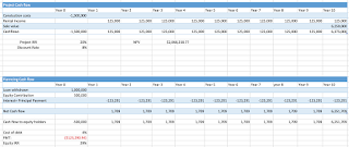
Here, we are trying to determine how sensitive our IRR analysis is to changes in initial costs or the annual rental revenue (our two main variables). To begin a sensitivity analysis we must first establish a base-case scenario. This is typically the IRR using assumptions we believe to be most accurate. Thereafter, we can change various assumptions we had initially made, based on other potential assumptions. IRR is then recalculated, and the sensitivity of the IRR based on the changes in assumptions is determined. This will be done for both the Project IRR and the Equity IRR.   
                           
To construct the matrix, follow the steps below. 

1. Reference your base assumption at 0% sensitivity level. This can be done by simply multiplying all cash flows in your initial IRR analysis by the cells that contain your sensitivity levels. In my preceding example, I added two cells C36 for the base revenue assumption and C37 for the base cost assumption- both at 0%. I then multiplied the initial cash outflow -1,500,00 *(1+C7); likewise, cells D8-M8 have all been multiplied by (1+C36). 

                                   

                                   

                                   

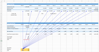
at this step, we are establishing that $1,500,00 is our base cost assumption with a 0% margin of error. Likewise,  $125,000 is our base revenue per year, assuming there is 0% variance in our predictions. 

2. In a cell on the worksheet, reference the formula that refers to the two input cells you want to sensitise. In the example, I referenced my project IRR in cell T66. 

3. Enter one list of input values in the same column, below the formula. In the example, I input a range of development cost possibilities i.e. I expect that the initial cost of construction will vary between -15% (best case) and +15% (worst case).

4. Enter the second list in the same row, to the right of the formula. I have input revenue growth assumptions, which again, I expect to fluctuate between -15% (worst case) and +15% (best case). 

5. Select the range of cells that contains the formula and both the row and column of values. In our example, I have selected T66:AA73.

6.  Click 'What-If analysis' tool under the 'Data Bar'. Select the 'Data table' from the options. Hit Alt-D-T on your keyboard for a shortcut on windows. 

7. In the row input cells box, enter the sensitivity level reference for the row. In my example, the rows represent the revenue income, hence, I selected cell C36 in the row input cell box. 

8. In the column input cells box, enter the sensitivity level reference for the column. In my example, the columns represent the cost of development, hence, I selected cell C37 in the column input cell box. 

9. Press OK! this will give us the different scenarios for the unleveraged IRR!

10. To compute the scenario analysis for leveraged IRR, repeat steps 2-9, just reference the formula for the leveraged IRR as the base cell you want to sensitise. 

                                          

                                           

Project IRR and Equity IRR Simplified

Executives, analysts, and investors often rely on internal-rate-of-return (IRR) calculations as one measure of a project’s yield. Real Estate Firms commonly use it as a shorthand benchmark to compare the relative attractiveness of diverse investments. The purpose of calculating the IRR is to determine if the rate of return of a project is greater than its cost of capital. Investments with the highest IRRs are considered the most attractive and are given higher priority.

Hypothetically speaking, IRR is defined as the discount rate which, when applied to discount a series of cash flows, results in a net present value equivalent to zero. An intuitive way of understanding IRR is to think of it as equivalent constant interest rate at which a given series of cash outflows must be invested in order for the investor to earn a given series of cash inflows as income. It is in this sense a measure of the underlying return the investor expects to achieve by investing in capital.

There are two useful classifications of IRR when making real-estate investment decisions; Project IRR and Equity IRR. A project’s IRR can be attained taking in consideration only the project’s cash flows (excluding the financing cash flows). Initially, IRR is determined at the project level, without considering cash flows related to financing i.e. when computing for the project IRR, amortisation and interest payments are excluded.

To illustrate, let's consider a project with an initial construction cost of $1,500,000, and annual rental income of $125,000. Assume after 10 years the property will be sold for $6,250,000. You can construct the project cash flows and calculate the project IRR by using the Excel IRR formula. From the calculation, we find the project has a 20% IRR and an NPV of  $2,068,258.77 at a discount rate of 8% as shown below.

                             

On the other hand, calculating Equity IRR is a different process. Equity IRR assumes the use debt to finance the investment, hence, any debt raised for the project is deducted from net cash inflows. However, if the project is fully funded by equity, the Project IRR and Equity IRR will be the same. If the project is fully funded by debt, Equity IRR simply does not exist. 

Let's assume that in our earlier example, 66.6% of the project is funded by debt while the remaining 33.3% is funded by equity. The cost of debt is 4%. The cash flows for equity holders and the equity IRR can be calculated using the same excel formula as above. We find that our Equity IRR is 29%. 

We can calculate the Interest + principlal payment using the following formula:

L[c(1+c)^n]/(1+C)^n-1]  

Where; 
L is the loan value  
C is Interest rate, and 
n is the number of payments.

Otherwise, we can use the PMT option in excel to calculate the principal payment. This option will ask you for arguments for the interest rate, number of payments, and the PV of the loan (the amount of the loan the day you withdrew it). 

A reoccurring question is whether the Equity IRR is always higher than the project IRR- the answer is no. The project IRR will be higher than the Equity IRR only when the cost of debt exceeds the Project's IRR. In our example, the project IRR will only exceed the Equity IRR if the cost of debt exceeds 20% (our project's IRR). 

In terms of the investment decision, a positive Equity IRR indicates that based on the set of assumptions used, the project under evaluation generates more than the required rate of return by investors, hence, the project should be accepted. Contrarily, a negative Equity IRR indicates that the project is unable to generate the required rate of return by investors, and hence, should be rejected. An Equity IRR of zero means that the project's rate of return is just equal to the cost of capital. The project would neither make you richer or poorer; it is worth what it costs. Thus the IRR rule states that the project should be accepted. Accordingly, our project under evaluation with Equity IRR of 29% should be accepted.